课程大纲
介绍
课程概览
课程包括的话题:
- Concepts of Function, Limits and Continuity 函数,极限,连续性的概念
- Differentiation Rules, Application to Graphing, Rates, Approximations, and Extremum Problems 微分规则,图形应用,比率,近似和极值问题
- Definite and Indefinite Integration 定积分和不定积分
- The Fundamental Theorem of Calculus 微积分基本定理
- Applications to Geometry: Area, Volume, and Arc Length 几何应用:面积,体积和弧长
- Applications to Science: Average Values, Work, and Probability 科学应用:平均值,功和概率
- Techniques of Integration 积分的技巧
- Approximation of Definite Integrals, Improper Integrals, and L’Hôspital’s Rule 定积分的近似值,瑕积分,洛必达法则
课程目标
完成此门课程后,应该对单变量微积分的基本概念和一系列技能有清晰的理解,能够有效地使用这些概念。
基础的概念如下:
- 导数(Derivative)(变化率),计算为比率的极限;
- 积分( Integral)(和),计算为黎曼和(Riemann sum)的极限。
需要拥有的能力:
- Use both the limit definition and rules of differentiation to differentiate functions.
- 使用极限定义和微分规则来区分函数。
- Sketch the graph of a function using asymptotes, critical points, the derivative test for increasing/decreasing functions, and concavity.
- 使用渐近线,临界点,增、减函数的导数测试和凹度绘制函数图形。
- Apply differentiation to solve applied max/min problems.
- 应用微分解决给定的最大、最小值问题。
- Apply differentiation to solve related rates problems.
- 应用微分解决相应的变化率问题。
- Evaluate integrals both by using Riemann sums and by using the Fundamental Theorem of Calculus.
- 通过使用黎曼和和微积分的基本定理来计算定积分的值。
- Apply integration to compute arc lengths, volumes of revolution and surface areas of revolution.
- 应用积分来计算弧长,旋转体积和旋转表面积。
- Evaluate integrals using advanced techniques of integration, such as inverse substitution, partial fractions and integration by parts.
- 使用高级定积分技巧来计算定积分,比如逆代换,部分分式积分,部分积分。
- Use L’Hospital’s rule to evaluate certain indefinite forms.
- 利用洛必达法则来计算某些不定型。
- Determine convergence/divergence of improper integrals and evaluate convergent improper integrals.
- 确定瑕积分的收敛或发散,然后计算收敛的瑕积分。
- Determine the convergence/divergence of an infinite series and find the Taylor series expansion of a function near a point.
- 确定无穷级数的收敛或发散,并找到一个点附近函数的泰勒级数展开。
1. 微分(DIFFERENTIATION)
Part A :定义和基础规则
Session 1:导数(Derivative)介绍
Clip 1
什么是导数?从几何解释( geometric interpretation)和物理解释(physical interpretation)分别展开来讲。
Clip 2 微分的几何解释
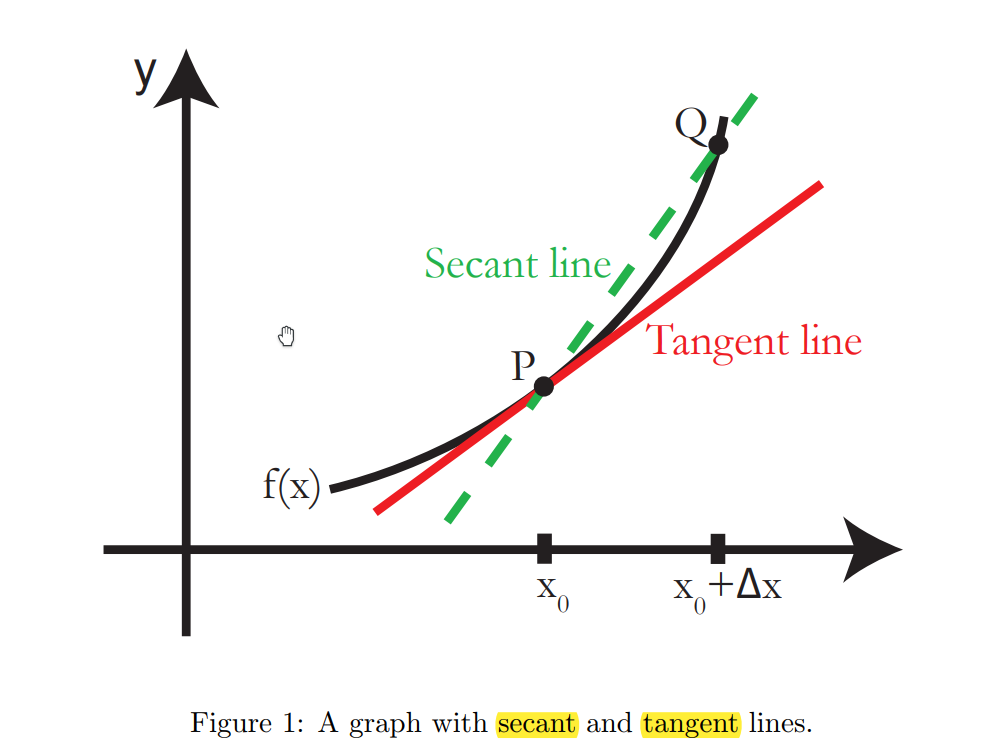
从几何上来看:
什么是切线(tangent line)?
- 不仅仅是与函数图像只有一个交点的直线;
- 也是函数$f(x)$的图像经过$P=(x_{0},f(x_{0})),Q$的割线(SECANT),当Q接近于P的极限。
同时,我们知道函数的公式时,可以通过点斜式和上述定义求出函数位于$P=(x_{0},f(x_{0}))$处的切线公式:
$y-y_{0} = m (x - x_{0})$,其中,$m = f^{‘}(x_{0})$。
Clip 3 割线的极限
割线是指与曲线图像有两个交点的直线。如果两个交点相距的非常近,那么,割线的斜率就与曲线的斜率近似相等。我们想要找到切线的斜率m—与曲线的斜率相等—那么可以利用割线的斜率来求出。
假设直线PQ是函数$f(x)$图像上的一条割线,函数图像在P点处的斜率,可以通过Q不断靠近P点的方式,由直线PQ的斜率求得。
(函数图像在P点处的)切线就等于当Q$\rightarrow$P时的割线PQ。
Clip 4 以比率作为斜率
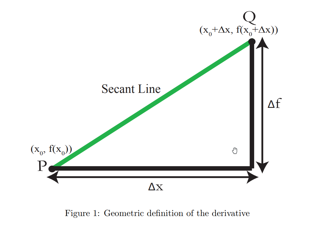
从函数$f(x)$的图像上一点$P(x_{0},f(x_{0})$,开始,水平移动一个很小的距离$\Delta x$,找到图像上另一点$Q(x_{0}+\Delta x,f(x_{0}+\Delta x))$,PQ即为函数图像的一条割线。P、Q两点的垂直距离$\Delta f = f(x_{0}+\Delta x) - f(x_{0})$。
由前述可知,切线是割线的极限,所以可知切线的斜率也是割线的斜率的极限。
割线的斜率,可由$\frac{\Delta f}{\Delta x}$。
所以,切线的斜率:
$m = \lim \limits_{Q \rightarrow P}{\Delta f \over \Delta x}=\lim\limits_{\Delta x \rightarrow 0}{\Delta f \over \Delta x}$
Clip 5 主要公式
由图中,可知$Q=(x_0+\Delta x,f(x_0+\Delta x))$,所以
切线和割线习题
(a)
| $\Delta{x}$ | -0.5 | -0.25 | 0.25 | 0.5 |
| :—————————————-: | :—-: | :—-: | :—-: | :—-: |
| $\frac{\Delta{x}}{\Delta{y}}$ | -0.53 | 0.16 | -0.41 | -0.59 |(b) $\frac{dy}{dx} = -0.16$
(c) $[-0.1,0.18]$
(a)
| $\Delta{x}$ | -0.5 | -0.25 | 0.25 | 0.5 |
| :—————————————-: | :—-: | :—-: | :—-: | :—-: |
| $\frac{\Delta{x}}{\Delta{y}}$ | -0.88 | -0.97 | -0.97 | -0.88 |(b) $\frac{dy}{dx} = -1.0$
(c) $[-0.46,0.46]$
(a)
| $\Delta{x}$ | -0.5 | -0.25 | 0.25 | 0.5 |
| :—————————————-: | :—-: | :—-: | :—: | :—: |
| $\frac{\Delta{x}}{\Delta{y}}$ | -0.59 | -0.41 | 0.16 | 0.53 |(b) $\frac{dy}{dx} = -0.16$
(c) $[-0.1,0.18]$
(a) 不一样;
额外的习题视频
$f(x) = \frac{1}{1+x^2}$,画出$f(x)$的图像,并求出$f^{‘}(x)$。
可以看出$f(x)$是一个偶函数,代入如下几个点,大致描绘出函数图像
| x | f(x) |
|---|---|
| -2 | 1/5 |
| -1 | 1/2 |
| 0 | 1 |
| 1 | 1/2 |
| 2 | 1/5 |
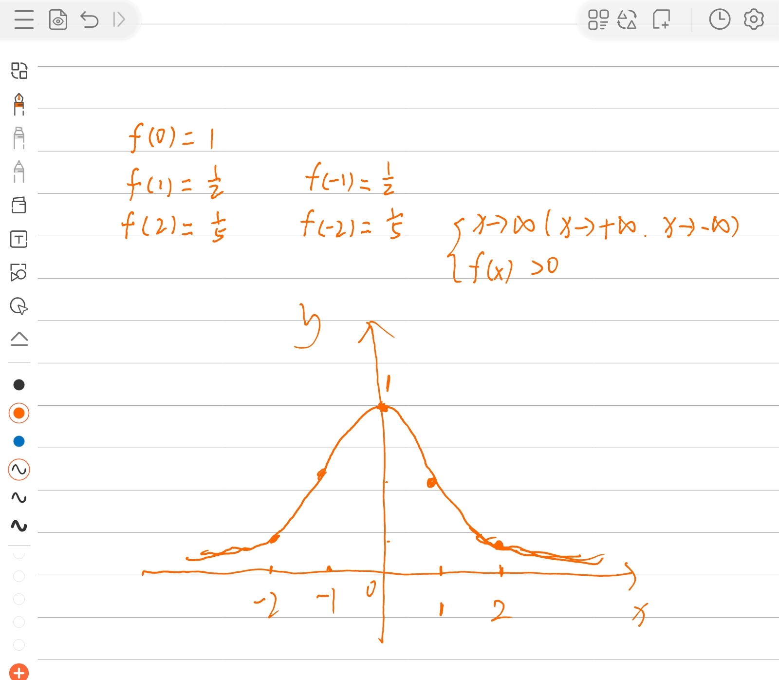
注意$x\rightarrow \infin (x \rightarrow +\infin 或者 x \rightarrow -\infin)$时,f(x)恒大于0.
导函数的图像
- 找出导数为0的点-原函数的顶点;
- 函数增区间,表示导数大于0;函数减区间,表示导数小于0;
- 距离导数为0的点最远的值也是图像最陡的地方,为导函数的顶点。
Session 2:导数举例
这一目将会运用主要公式来求函数$\frac{1}{x}和x^n$的导数。并且学习导数的另一种书写方式。
Clip 1 例子1 y=1/x
Clip 2 难题:位于y=1/x的图像下的三角形
Clip 3 导数表示方法
Clip 4 y=x^n
二项式定理: